<?xml version="1.0" encoding="utf-8"?><feed xmlns="http://www.w3.org/2005/Atom" ><generator uri="https://jekyllrb.com/" version="3.10.0">Jekyll</generator><link href="https://ovcharenkoo.com/feed.xml" rel="self" type="application/atom+xml" /><link href="https://ovcharenkoo.com/" rel="alternate" type="text/html" /><updated>2026-05-16T05:19:04+00:00</updated><id>https://ovcharenkoo.com/feed.xml</id><title type="html">Oleg Ovcharenko</title><subtitle>AI &amp; Energy expert at NVIDIA specializing in industrial agentic AI, Large Language Models, and HPC applications for oil &amp; gas and renewable energy sectors</subtitle><author><name>Oleg Ovcharenko, PhD</name><email>oleg.ovcharenko@kaust.edu.sa</email></author><entry><title type="html">Useful commands for data processing in Madagascar</title><link href="https://ovcharenkoo.com/Madagascar/" rel="alternate" type="text/html" title="Useful commands for data processing in Madagascar" /><published>2019-07-09T00:00:00+00:00</published><updated>2019-07-09T00:00:00+00:00</updated><id>https://ovcharenkoo.com/Madagascar</id><content type="html" xml:base="https://ovcharenkoo.com/Madagascar/"><![CDATA[<h2 id="segy-to-rsf">Segy to RSF</h2>

<div class="language-plaintext highlighter-rouge"><div class="highlight"><pre class="highlight"><code>sfsegyread &lt; file.sgy &gt; file.rsf
</code></pre></div></div>

<h2 id="plot-from-rsf">Plot from .rsf</h2>
<div class="language-plaintext highlighter-rouge"><div class="highlight"><pre class="highlight"><code>sfgrey &lt; file.rsf | sfpen if complex, pipe ```| sfreal | sfpen```
</code></pre></div></div>

<h2 id="brief-about-the-rsf">Brief about the .rsf</h2>
<div class="language-plaintext highlighter-rouge"><div class="highlight"><pre class="highlight"><code>sfin &lt; file.rsf
</code></pre></div></div>

<h2 id="crop-window-from-rsf">Crop window from .rsf</h2>
<div class="language-plaintext highlighter-rouge"><div class="highlight"><pre class="highlight"><code> sfwindow &lt; file.rsf n1=2000 n2=500 &gt; file2.rsf
</code></pre></div></div>

<p><code class="language-plaintext highlighter-rouge">Example: sfwindow &lt; file.rsf n1=2000 n2=500 | sfgrey | sfpen</code></p>]]></content><author><name>Oleg Ovcharenko, PhD</name><email>oleg.ovcharenko@kaust.edu.sa</email></author><category term="Madagascar" /><summary type="html"><![CDATA[Quick reference guide for Madagascar seismic processing software - commands for reading SEGY files, plotting RSF data, and windowing operations]]></summary></entry><entry><title type="html">Notes on finite-difference wave propagation</title><link href="https://ovcharenkoo.com/fd_facts/" rel="alternate" type="text/html" title="Notes on finite-difference wave propagation" /><published>2018-03-20T00:00:00+00:00</published><updated>2018-03-20T00:00:00+00:00</updated><id>https://ovcharenkoo.com/fd_facts</id><content type="html" xml:base="https://ovcharenkoo.com/fd_facts/"><![CDATA[<h2 id="finite-difference-method">Finite-difference method</h2>

<p>“If one wants to solve an ODE or PDE to high accuracy on a simple domain, and if the data defining the problem are smooth, then spectral methods are usually the best tool. They can often achieve ten digits of accuracy where a finite-difference or finite element method would get two or three. At lower accuracies, they demand less computer memory than the alternatives.” Trefethen (2000)</p>

<!-- @trefethen2000spectral -->

<table>
  <thead>
    <tr>
      <th>O(T,S)</th>
      <th>Medium</th>
      <th>PPW</th>
      <th>PD</th>
      <th>Reference</th>
    </tr>
  </thead>
  <tbody>
    <tr>
      <td>2-2</td>
      <td>Homo</td>
      <td>10</td>
      <td>10</td>
      <td>(Kelly et al., 1976)</td>
    </tr>
    <tr>
      <td>2-4</td>
      <td>Homo</td>
      <td>5</td>
      <td>30</td>
      <td>(Levander, 1989)</td>
    </tr>
    <tr>
      <td>2-2</td>
      <td>Heter</td>
      <td>15-20</td>
      <td>10</td>
      <td> </td>
    </tr>
    <tr>
      <td>2-4</td>
      <td>Heter</td>
      <td>10-15</td>
      <td>30</td>
      <td> </td>
    </tr>
  </tbody>
</table>

<p>where O(T,S) is order of accuracy in time and space,  PPW is number of points per wavelength and PD is propagation distance in terms of wavelength.</p>

<p>If the gridpoint spacing is too coarse, dipping interfaces appear as stair-steps, where the edge of each step acts as a strong diffractor. If the waves propagate more than 30 wavelengths, empirical evidence suggests higher-order schemes of 2-8 or higher are needed.  Stork (2013) claims that numerical dispersion errors should be no more than π/20 after propagating more than 50 wavelengths, which is equivalent to a 0.05% phase error. Otherwise there can be a fatal buildup of errors when iterative methods such as FWI or least squares migration are used. He suggests that longer 25-point stencils using optimized coefficients (Zhang and Yao, 2013) are much better at controlling numerical dispersion.</p>

<p>Today’s best practice is to use higher-order finite-difference stencils, with recommendations of <strong>8th-order in space and 2nd-order in time</strong>. For media with strong contrasts in physical properties (water next to elastic sediments or air), the staggered grid scheme is recommended over the conventional FD solutions to the second-order wave equation.</p>

<h2 id="pseudospectral-method">Pseudospectral method</h2>

<p>Spatial derivative in the Fourier domain. (Kreiss and Oliger, 1972; Kosloff and Baysal, 1982; Kosloff et al., 1982). In theory, only <strong>two points per wavelength</strong> are needed for an accurate solution in a smooth medium.</p>

<p>ince the FFT represents the derivative in the wavenumber domain by the exact multiplication of ikx, then its spatial representation is equivalent to a discrete derivative operator that is as wide as the computational domain. It requires a periodic boundary condition, but if the absorbing boundary conditions are effective (see Appendix 8.9 and Liu and Sen (2010, 2012)) then this should not be a problem.</p>

<h2 id="spectral-element-vs-finite-element">Spectral Element VS Finite Element</h2>

<p>The SE method differs from the standard FE element in that its nodes are at the <strong>unevenly spaced quadrature points (GLL)</strong>, and therefore removes the need to make the lumped mass approximation.</p>

<h2 id="sponge-boundary">Sponge boundary</h2>

<p>The simplest absorbing boundary condition is that of a damping zone (Cerjan et al., 1985), also known as a sponge zone, with a <strong>thickness of about 5-10 wavelengths</strong> located next to the sides of the model. Inside the leftside sponge region the wavefield is multiplied by an exponential damping function f(i) at each time step, where i is the gridpoint index for the x-coordinate. A modified damping function is proposed by Wang and Qin (1997)</p>

<p>For staggered grid, damping just the particle-velocity component after each time step is less effective than damping both the stress and particle-velocity components after each time step. However, an instability has been observed when both stress and velocity components are damped for the elastic wave equation.</p>

<h2 id="viscoelasticiy">Viscoelasticiy</h2>

<p>For a viscoelastic fluid, the <strong>Maxwell model</strong> predicts that stress decays exponentially to zero, which is accurate <strong>for a viscoelastic fluid</strong>, not a solid.</p>]]></content><author><name>Oleg Ovcharenko, PhD</name><email>oleg.ovcharenko@kaust.edu.sa</email></author><category term="FD" /><summary type="html"><![CDATA[Technical notes on finite-difference time-domain methods for wave propagation, including accuracy requirements, spectral methods, and boundary conditions for seismic modeling]]></summary></entry><entry><title type="html">Install Keras with Tensorflow backend and GPU support in Anaconda</title><link href="https://ovcharenkoo.com/install-keras-anaconda-gpu/" rel="alternate" type="text/html" title="Install Keras with Tensorflow backend and GPU support in Anaconda" /><published>2018-01-03T00:00:00+00:00</published><updated>2018-01-03T00:00:00+00:00</updated><id>https://ovcharenkoo.com/install-keras-anaconda-gpu</id><content type="html" xml:base="https://ovcharenkoo.com/install-keras-anaconda-gpu/"><![CDATA[<ol>
  <li>Install Nvidia driver</li>
  <li>Install Cuda</li>
  <li>Install cuDNN</li>
  <li>Install Anaconda</li>
  <li>Open terminal and type one-by-one the following commands
    <div class="language-plaintext highlighter-rouge"><div class="highlight"><pre class="highlight"><code>conda create -n EnvName python=3.6 pip spyder
conda install -n EnvName tensorflow-gpu
conda install -n EnvName -c conda-forge keras-gpu
</code></pre></div>    </div>
  </li>
</ol>

<p>Use it</p>

<div class="language-plaintext highlighter-rouge"><div class="highlight"><pre class="highlight"><code>source activate EnvName
spyder . &amp;
</code></pre></div></div>

<p>Done.</p>]]></content><author><name>Oleg Ovcharenko, PhD</name><email>oleg.ovcharenko@kaust.edu.sa</email></author><category term="Tensorflow" /><category term="Keras" /><category term="GPU" /><category term="Anaconda" /><summary type="html"><![CDATA[Step-by-step tutorial for installing Keras with TensorFlow GPU backend in Anaconda environment, including CUDA, cuDNN setup, and conda environment configuration]]></summary></entry><entry><title type="html">Compare Latex documents with latexdiff on Mac</title><link href="https://ovcharenkoo.com/latexdiff/" rel="alternate" type="text/html" title="Compare Latex documents with latexdiff on Mac" /><published>2017-12-21T00:00:00+00:00</published><updated>2017-12-21T00:00:00+00:00</updated><id>https://ovcharenkoo.com/latexdiff</id><content type="html" xml:base="https://ovcharenkoo.com/latexdiff/"><![CDATA[<p>Quick comparison of two Latex documents</p>

<div class="language-plaintext highlighter-rouge"><div class="highlight"><pre class="highlight"><code>latexdiff ../path/old.tex new.tex --flatten &gt; diff.tex
</code></pre></div></div>

<p><code class="language-plaintext highlighter-rouge">--flatten</code> here means to unwrap all included files into a flat text</p>

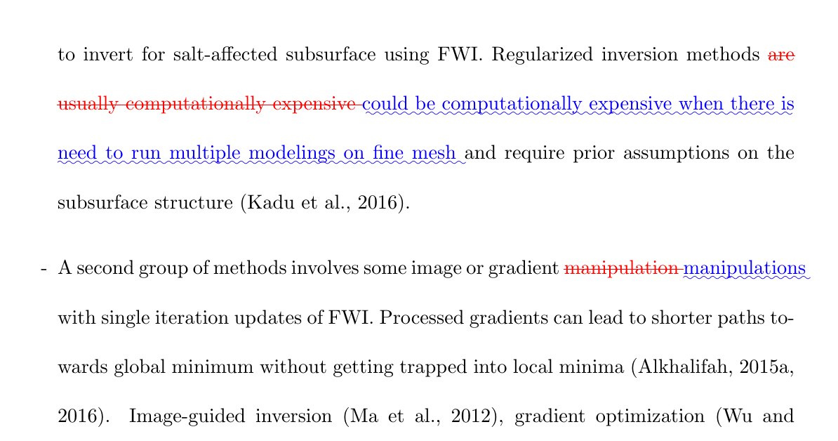
<p>At the end the difference looks like this:
<img src="/assets/images/latexdiff.png" alt="Result" /></p>

<p>Beware that sometimes the resulting <code class="language-plaintext highlighter-rouge">diff.tex</code> file is compiled with errors. Usually they are resolved by removing preceeding the error empty lines or adding <code class="language-plaintext highlighter-rouge">$</code> arround math symbols.</p>]]></content><author><name>Oleg Ovcharenko, PhD</name><email>oleg.ovcharenko@kaust.edu.sa</email></author><category term="Latex" /><summary type="html"><![CDATA[Quick guide to using latexdiff command-line tool on Mac for comparing and highlighting differences between LaTeX document versions]]></summary></entry><entry><title type="html">Transparent background when saving figures in Matlab (e.g png, eps etc.)</title><link href="https://ovcharenkoo.com/transparent-background/" rel="alternate" type="text/html" title="Transparent background when saving figures in Matlab (e.g png, eps etc.)" /><published>2017-11-09T00:00:00+00:00</published><updated>2017-11-09T00:00:00+00:00</updated><id>https://ovcharenkoo.com/transparent-background</id><content type="html" xml:base="https://ovcharenkoo.com/transparent-background/"><![CDATA[<p>Often you need to generate multiple figures with transparent background in order to put them directly into TeX document or presentation, but Matlab is prone to saving with white background using <code class="language-plaintext highlighter-rouge">print</code></p>

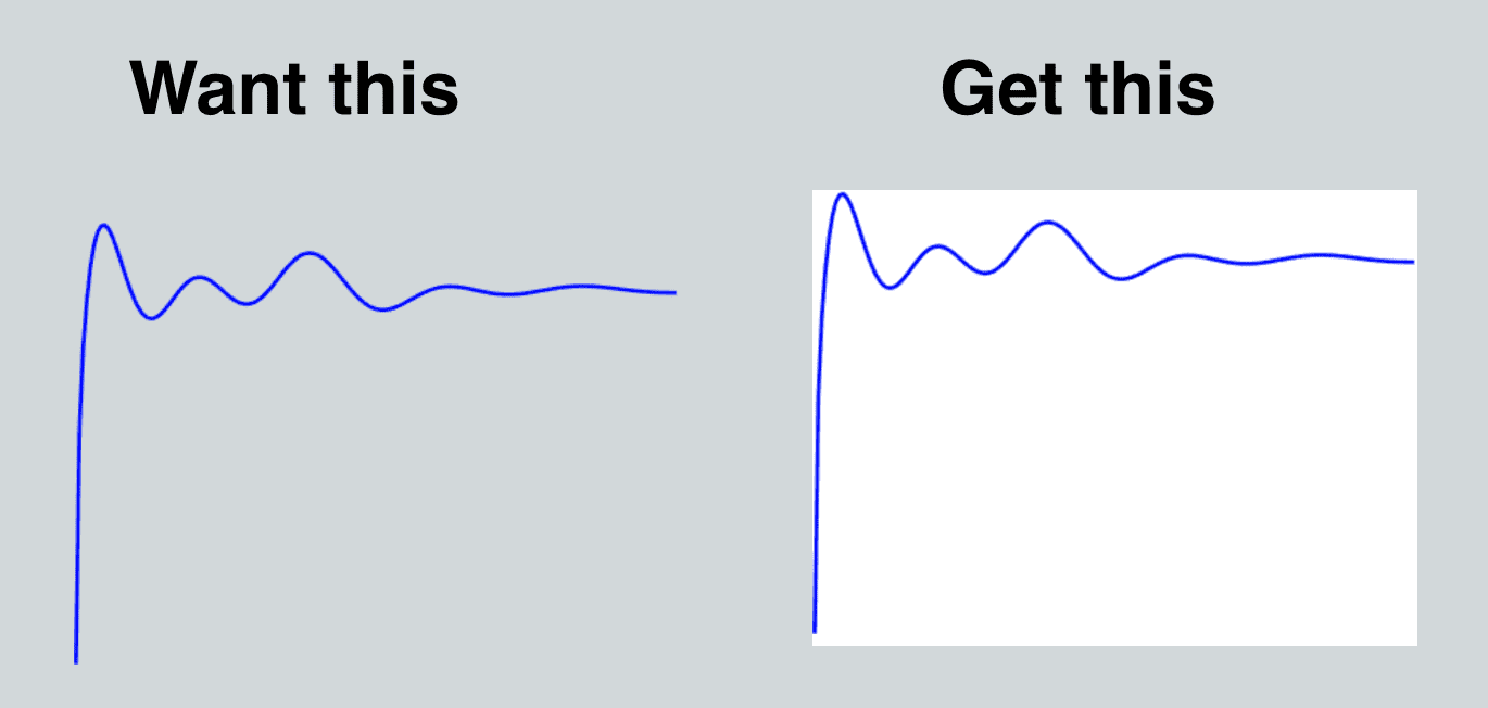
<h2 id="problem">Problem:</h2>
<p><img src="/assets/images/transparent_background.png" alt="Transparent vs non-transparent  background" /></p>

<h2 id="solution">Solution:</h2>
<p>Use <a href="http://www.mathworks.com/matlabcentral/fileexchange/23629-export-fig">export_fig</a> by Yair Altman.</p>

<p>“This function saves a figure or single axes to one or more vector and/or bitmap file formats, and/or outputs a rasterized version to the workspace, with the following properties</p>

<ul>
  <li>Figure/axes reproduced as it appears on screen</li>
  <li>Cropped/padded borders (optional)</li>
  <li>Embedded fonts (pdf only)</li>
  <li>Improved line and grid line styles</li>
  <li>Anti-aliased graphics (bitmap formats)</li>
  <li>Render images at native resolution (optional for bitmap formats)</li>
  <li>Transparent background supported (pdf, eps, png, tiff)</li>
  <li>Semi-transparent patch objects supported (png, tiff)</li>
  <li>RGB, CMYK or grayscale output (CMYK only with pdf, eps, tiff)</li>
  <li>Variable image compression, including lossless (pdf, eps, jpg)</li>
  <li>Optional rounded line-caps (pdf, eps)</li>
  <li>Optionally append to file (pdf, tiff)</li>
  <li>Vector formats: pdf, eps</li>
  <li>Bitmap formats: png, tiff, jpg, bmp, export to workspace”</li>
</ul>

<h2 id="how-to">HOW TO</h2>

<ol>
  <li>Download the package from <a href="http://www.mathworks.com/matlabcentral/fileexchange/23629-export-fig">here</a> (sign in if required)</li>
  <li>Unzip it and place to the folder with your project (rename it if needed e.g. to <em>export_fig_folder</em>)</li>
  <li>Add the folder to path by <em>Right Click -&gt; Add to path -&gt; Selected folders and subfolders</em>, or by adding <code class="language-plaintext highlighter-rouge">addpath('./export_fig_folder/')</code> to your script</li>
</ol>

<p>Use function in the following manner:</p>

<p>Add <code class="language-plaintext highlighter-rouge">set(gcf, 'Color', 'None')</code> to your figure property or <code class="language-plaintext highlighter-rouge">-transparent</code> key when calling function</p>

<div class="language-plaintext highlighter-rouge"><div class="highlight"><pre class="highlight"><code>save_path = '../pics/MyPic';
export_fig(save_path, '-png', '-eps', '-transparent');
</code></pre></div></div>

<p>or:</p>

<div class="language-plaintext highlighter-rouge"><div class="highlight"><pre class="highlight"><code>export_fig ../pics/MyPic -png -eps -transparent;
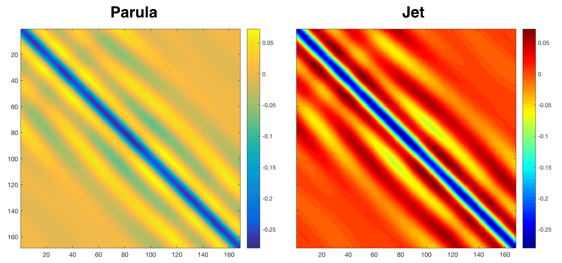
</code></pre></div></div>]]></content><author><name>Oleg Ovcharenko, PhD</name><email>oleg.ovcharenko@kaust.edu.sa</email></author><category term="Matlab" /><summary type="html"><![CDATA[Tutorial on saving MATLAB figures with transparent backgrounds using export_fig function for PNG, EPS, PDF formats - perfect for presentations and LaTeX documents]]></summary></entry><entry><title type="html">How to set Matlab default colormap</title><link href="https://ovcharenkoo.com/matlab-default-colormap/" rel="alternate" type="text/html" title="How to set Matlab default colormap" /><published>2017-10-09T00:00:00+00:00</published><updated>2017-10-09T00:00:00+00:00</updated><id>https://ovcharenkoo.com/matlab-default-colormap</id><content type="html" xml:base="https://ovcharenkoo.com/matlab-default-colormap/"><![CDATA[<p>Standard Matlab colormap <em>parula</em> is pretty nice, but I used to <em>jet</em> and it is tedious to add colormap(jet) everywhere manually. The simple way is to change the default colormap:</p>

<p><img src="/assets/images/parula_vs_jet.png" alt="*Parula* and *Jet* colormaps" /></p>

<div class="language-plaintext highlighter-rouge"><div class="highlight"><pre class="highlight"><code>set(groot,'DefaultFigureColormap',jet)
</code></pre></div></div>

<p><a href="https://www.mathworks.com/matlabcentral/answers/246461-how-can-i-get-the-default-colormap-to-be-jet-in-matlab-2014b">Source</a></p>]]></content><author><name>Oleg Ovcharenko, PhD</name><email>oleg.ovcharenko@kaust.edu.sa</email></author><category term="Matlab" /><summary type="html"><![CDATA[Quick tip for changing MATLAB's default colormap from Parula to Jet or any other colormap using set(groot) command]]></summary></entry></feed>